CS 272: Foundations of Learning, Decisions, and Games
Table of Contents
- Lecture 2: Statistical Learning I (September 2nd, 2025)
- Lecture 3: Statistical Learning II (September 4th, 2025)
- Lecture 4: Statistical Learning III (September 9th, 2025)
- Lecture 5: Online Learning I (September 11th, 2025)
- Lecture 6: Online Learning II (September 16th, 2025)
- Lecture 7: Online Learning III (September 18th, 2025)
- Lecture 8: Learning with Smoothed Adversaries I (September 23rd, 2025)
- Lecture 9: Learning with Smoothed Adversaries II (September 25th, 2025)
- Lecture 10: Bandits and Partial Feedback (September 30th, 2025)
- Lecture 11: Zero-Sum Games (October 2, 2025)
- Lecture 12: General-Sum Games and Nash Equilibria (October 7, 2025)
- Lecture 13: Correlated Equilibria (October 9, 2025)
- Lecture 14: Auctions (October 14, 2025)
Notes for Nika Haghtalab’s Fall 2025 course. A work in progress.
Lecture 2: Statistical Learning I (September 2nd, 2025)
- What is an algorithm that learns the class of 2D axis-aligned rectangles in the consistency model? What is the runtime of such an algorithm?
- What is True Error? What is Empirical Error?
- When does an algorithm PAC-learn a concept class? What is the difference between proper and improper PAC-learnability?
- Prove the PAC-learnability of finite concept classes.
Defining a Formal Model for Statistical Learning
- Domain, $\mathcal X$, the set of all possible instances. Each instance is vector of features.
- Label set, $\mathcal Y$. Assume for now that $\mathcal Y = \set{0, 1}$.
- Concept class, $\mathcal C$, where a concept is a mapping $c: \mathcal X \to \mathcal Y$. Example concepts: Boolean expressions of the features, look-up tables, etc. A concept class is a restriction on the search space of possible classifiers.
The Consistency Model
Definition (Consistency). A concept, $c$, is consistent with a set of samples, $S = \lbrace (x_1, y_1), \ldots (x_m, y_m) \rbrace$, if $c(x_i) = y_i$ for all samples in $S$.
In the Consistency Model, an algorithm $\mathcal A$ learns $\mathcal C$ if, given $S$,
\[\mathcal A(S) = \begin{cases}c \quad \text{such that $c$ is consistent with }S\\ \text{DNE}\quad \text{if no such $c \in \mathcal C$}\end{cases}\]Training Data
The training data for an algorithm is $S \subseteq \mathcal X \times \mathcal Y$. Often, it is assumed that this training data is sampled IID from a data distribution, $\mathcal D$, which is a probability distribution over $\mathcal X$. For now, assume there exists a true labeling function, $f(x)$, where $f: \mathcal X \to \mathcal Y$.
Assumption (Realizability of $\mathcal C$). Under the Realizability Assumption, there exists a concept, $c \in \mathcal C$, such that $\text{err}_{(\mathcal D, f)} = 0$. It follows that $c(x_i) = f(x_i) = y_i$ for all $(x_i, y_i) \in S$, so $\text{err}_S(c) = 0$.
Both $\mathcal D$ and $f(x)$ are unknown to the learning algorithm, $\mathcal A$.
Measures of Error
Definition (True Error). The True Error is calculated over the data distribution, and is defined as
\[\text{err}_{\mathcal D}(c) = \mathbb P \left[ c(x) \neq f(x) \right]\]
Definition (Empirical Error). The Empirical Error is calculated over the training data, and is defined as
\[\text{err}_S(c) = \frac{1}{m} \sum_{i=1}^m \mathbb 1\set{c(x_i) \neq y_i}\]
PAC-Learnability
Conceptually, a finite concept class $\mathcal C$ is PAC-learnable if a sufficiently accurate classifier can be learned, with sufficiently high probability, given a sufficiently large training dataset.
Definition (PAC-Learnability). Formally, a finite concept class $\mathcal C$ is PAC-learnable if $\exists m: (0, 1)^2 \to \mathbb N$ such that, for any $(\epsilon, \delta) \in (0, 1)^2$ and $(\mathcal D, f)$ where Realizability of $\mathcal C$ with respect to $(\mathcal D, f)$ holds, $\exists \mathcal A$ such that, given $S$ where $\lvert S \rvert \geq m(\epsilon, \delta)$, $\mathcal A(S) = c$ where $\text{err}_{(\mathcal D, f)}(c) \leq \epsilon$ with probability at least $1 - \delta$.
Theorem (PAC-Learnability of Finite Concept Classes). If $\mathcal A$ learns $\mathcal C$ in the Consistency Model, where $\mathcal C$ is a finite concept class, then $\mathcal A$ PAC-learns $\mathcal C$ with number of samples
\[m(\varepsilon, \delta) = \mathcal O\left(\frac{\ln(|C|/\delta)}{\varepsilon} \right)\]Lecture 3: Statistical Learning II (September 4th, 2025)
- What is the projection of a concept class, $\mathcal C$, on a sample set, $S$?
- What is a growth function? Consider the example for 2D axis-aligned rectangles.
- What is the Fundamental Theorem of PAC-Learning?
- What is the Multiplicative Chernoff Bound? McDiarmid Inequality? Hoeffding Bound?
- What is a graph clique?
Growth Functions
Definition (Growth Function). For a concept class, $\mathcal C$, and sample complexity, $m$, \(\Pi_{\mathcal C}(m) = \max_{C \subseteq \mathcal X, |C| = m} |\mathcal C_C|\)
Example. What is $\Pi_{\mathcal C}(m)$, where $\mathcal C$ consists of functions $c: \mathcal X \to \set{0, 1}$?
Answer.
$2^m$.Example. What is $\Pi_{\mathcal C}(m)$, where $\mathcal C$ consists of intervals defined in one dimension?
Example. What is $\Pi_{\mathcal C}(m)$, where $\mathcal C$ consists of axis-aligned rectangles defined in two dimensions?
Fundamental Theorem of PAC Learning
Theorem. if $\mathcal A$ learns $\mathcal C$ in the consistency model, it also learns $\mathcal C$ in the PAC model so long as
\[m \geq \frac{2}{\varepsilon}\left(\log \Pi_{\mathcal C}(2m) + \log\frac{2}{\delta}\right)\]Lecture 4: Statistical Learning III (September 9th, 2025)
Note that hypothesis class, $\mathcal H$, and concept class, $\mathcal C$, are used interchangeably here. Restriction and projection are also used interchangeably. I’ll fix this later.
- Prove that there exists an infinite-sized hypothesis class that is PAC-learnable.
- What is the restriction of $\mathcal H$ on $C$?
- When does $\mathcal H$ shatter $C$? If $\mathcal H$ shatters $C$, what can be said about the learnability of $\mathcal H$?
- What is VC Dimension? How does it characterize learnability?
- What are the bounds on VC Dimension for a finite hypothesis class?
- What is the Fundamental Theorem of PAC Learning, given in terms of VC Dimension?
No-Free-Lunch
There does not exist a universal learner. For an unrestricted hypothesis class, given a hypothesis, $h$, it’s possible to adversarially construct a task on which it fails.
Shattering
Definition. A hypothesis class, $\mathcal H$, shatters $C \subseteq \mathcal X$ if $ \mathcal H_{C} = 2^{ C }$.
VC Dimension
Definition. The VC dimension of a hypothesis class is the size of the largest $C \subset \mathcal X$ that the hypothesis class can shatter.
If $\text{VCDim}(\mathcal H) < \infty$, $\mathcal H$ is PAC-learnable. If $\text{VCDim}(\mathcal H) = \infty$, $\mathcal H$ is able to shatter sets of arbitrarily large size, and $\mathcal H$ is not PAC-learnable.
Example. Consider the hypothesis class of threshold functions, $\mathcal H = \set{h_a(x) = \mathbb 1\set{x < a} | a \in \mathbb R}$. Is it PAC-learnable?
Answer.
Consider the restriction $\mathcal H_{C_1}$, where $C_1 = \set{c_1}$. $\mathcal H_{C_1} = \set{(0), (1)}$, which is indeed the set of all mappings $C_1 \to \set{0, 1}$. Thus, $\mathcal H$ shatters a set with size 1.Consider the restriction $\mathcal H_{C_2}$, where $C_2 = \set{c_1, c_2}$ such that $c_1 \leq c_2$. $\mathcal H_{C_2} = \set{(0, 0), (1, 0), (1, 1)}$, which does not satisfy $|\mathcal H_{C_2}| = 2^{|C|} = 4$. Thus, $\mathcal H$ does not shatter a set with size 2. Conclude that $\text{VCDim}(\mathcal H) = 1$, which is finite. Therefore, $\mathcal H$ is PAC-learnable.
Sauer’s Lemma
Lemma. If $\text{VCDim}(\mathcal H) \leq d < \infty$, then, $\forall m$,
\[\Pi_{\mathcal H}(m) \leq \sum_{i=0}^d \binom{m}{i}\]If $m > d+1$, then $\Pi_{\mathcal H}(m) \leq \left(\frac{em}{d}\right)^d$.
Lecture 5: Online Learning I (September 11th, 2025)
- Mistake bound model
Lecture 6: Online Learning II (September 16th, 2025)
- Relax consistency assumption
- What is the Majority/Halving Algorithm?
- Weighted Majority Algorithm
- $n$ experts, don’t want to regret not listening to a recommendation
- cost function, adversary
- alg cost close to opt cost as much as possible
- randomized weighted majority
Theorem. For any $T > 0$, adaptive adversary, for random weighted majority
\[\mathbb E \sum_{t=1}^T c^t(i^t) < \frac{1}{1-\epsilon}\mathbb E \min_{i \in [n]} \sum_{t=1}^T c^t(i) + \frac{1}{\epsilon} \ln n\] \[\ln (W^{t+1}) \leq \ln n - \epsilon \mathbb E \sum_{t=1}^T c^t (i^t)\]Lecture 7: Online Learning III (September 18th, 2025)
Lecture 8: Learning with Smoothed Adversaries I (September 23rd, 2025)
Lecture 9: Learning with Smoothed Adversaries II (September 25th, 2025)
- FTPL, FTRL
- hallucinated history
- pertubation term in the cost - how much does the hallucination matter? expectation of regret
Lecture 10: Bandits and Partial Feedback (September 30th, 2025)
- In a typical classification setting, experts $i \in [n]$, see $c^t(i) \forall i \in [n]$
- where the experts are possible hypotheses, $h_1, \ldots, h_n$
- unrealistic in the setting where you can see the cost everywhere, for example:
- traffic
- pricing - you do see lower half
- regret: $\sqrt{T \ln n}$
Partial Information
- versions of multi-armed bandit
- $E_i = \set i$
- $E_i = [n]$ - full information, which is the previous setting
- other results:
- apple-tasting
- feedback graphs
- what is the dependence of regret on $n$, $T$, in multi-armed bandits?
- exploration
-
penalization needs to account for likelihood of being picked
- EXP3 Algorithm - old school, exponential weights for exploration and exploitaition
- hyperparameter, $\gamma$, with ssome partial probability, choose expert with uniform randomness \(q_i^t = (1- \gamma) \frac{w_i^t}{\sum w_j^t} + \frac{\gamma}{n}\)
- cost only non-zero for experts played
\(\hat c^t = [0, \ldots, \frac{c(i^t)}{q_{i^t}}, 0, \ldots, 0]\)
Lecture 11: Zero-Sum Games (October 2, 2025)
- What is the Old School EXP3 algorithm?
- What is the regret calculation, when using utility instead of cost?
- When $\gamma = \sqrt{\frac{n \ln n}{T}}$, what is the expected regret of EXP3?
- The proof is similar to the multiplicative weights proof.
Theorem. When $\gamma = \epsilon$,
\[\mathbb E \sum u^t(i^t) \geq (1 - \gamma)\mathbb E \max_i \sum u^f(i) - \frac{n}{\gamma} \ln n\]The LHS is ALG, the RHS is OPT - an exploration term.
- In general, can’t use Linearity of Expectation for expectation over a max or min.
- RWM is a no regret algorithm.
RWM Facts
Claim 3.
- What is the modification made to the theorem to reduce it to the full information setting? (EXP3’).
- How to reduce to Randomized Weighted Majority? What is the range of utility values?
- How to prove the theorem for the modified setting?
- What is $\hat u^t (j)$ an unbiased estimator of? Prove it.
- Prove the second fact, that $\hat{\text{OPT}}$ in RWM is more competitive then OPT (the best expert according to utilities $u$).
- Prove the third fact.
- Prove the fourth fact, that EXP3’ reward is large fraction of RWM reward.
New School EXP3
Shown that uniform exploration is not necessary. The new school algorithm, then, uses the update rule
\[q_i^t \leftarrow p^t_i - \frac{w_i^t}{\sum_{i=1}^n w_i^t}\]Doesn’t have an explicit exploration term, but the randomness of choosing a random expert provides sufficient exploration.
Without full information, regret scales with the number of experts.
Games
For example, rock-paper-scissors. Game can be represented as a pay-off matrix between the row and column players.
Formally, a game consists of
- $m$ players, and their action sets $A_1, \ldots, A_m$.
- Utilities of players, $u_1, \ldots, u_m$.
Definition (Zero-Sum Game). Only two players, $u_1(a_1, a_2) = -u_2(a_1, a_2)$.
Strategies can be pure or mixed. In general, for a mixed strategry profile $p_1, \ldots, p_m$
- What is the bilinear form of utility for a Zero-Sum Game?
Theorem (Min-Max Theorem).
\[\text{Value of Game} = \max_p \min_q p^\intercal U q = \min_q \max_p p^\intercal U q\]It doesn’t matter if you start first!
Proof. This proof is from the 1990s. Term the LHS as $A$, and the RHS as $B$. $A \leq B$ is easy to see! (Prove using Jensen’s.) Because going second is better.
To show $A \geq B$, construct two intermediate points using the No Regret algorithm.
Lecture 12: General-Sum Games and Nash Equilibria (October 7, 2025)
Zero-Sum vs. General-Sum Games
Definition (Payoff). $U_i(p) = \mathbb E_{\forall i, a_i \sim p_i} U_i(a)$.
- for zero-sum games, there is a notion of “optimality” via min-max theorem, this notion of optimality often doesn’t exist in general-sum games
Definition (Optimality). $p^$ is maxmin optimal if $\forall q, U(p^, q) \geq \text{Val}$. $q^$ is minmax optimal if $\forall p, U(p, q^) \leq \text{Val}$.
- equilibria: stability where agents don’t deviate from strategy
Prisoner’s Dilemma
First example of general-sum game. Each thief has two options: confess, do not confess.
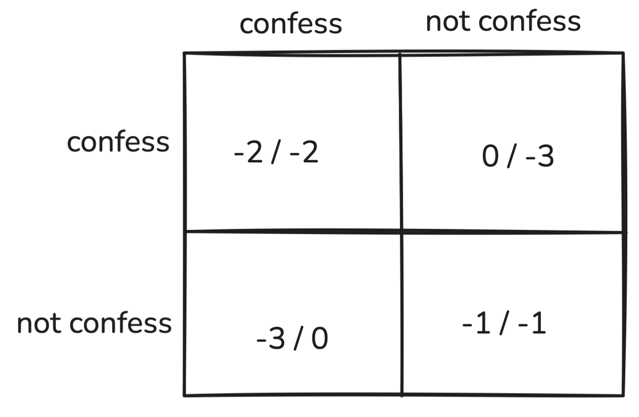
“Confessing” is the dominant strategy for both players. Regardless what the row player does, the payoff is always better if the column player confesses, and vice versa.
Definition (Dominant Strategy). Regardless of what the other player does, there is a pure strategy that is better.
Definition (Dominant Strategy Equilibria).
- doesn’t always exist, sometimes, what yo uplay depends on what other people are playing
- can you have a mixed dominant strategy?
Nash Equilibrium
mixed strategy $p$ is MNE iff
- any DSE is a NE
-
NE always exists, when finite utility, finite players
- in HW4, any minmax eq is also nash eq
- DSE \subset PNE \subset MNE
False statement: if p* MNE \implies all gradients of p* are 0
True statement: if all gradients are zero \implies p* is MNE
convex-concave game, no badly behaved saddle points because of bliniear nature of the payoff
Theorem. every game, finite # players & finite utilities between 0 and 1 has MNE (non necessarily PNE)
theorem
- brower’s fixed point
- berg’s theorem